Introducción

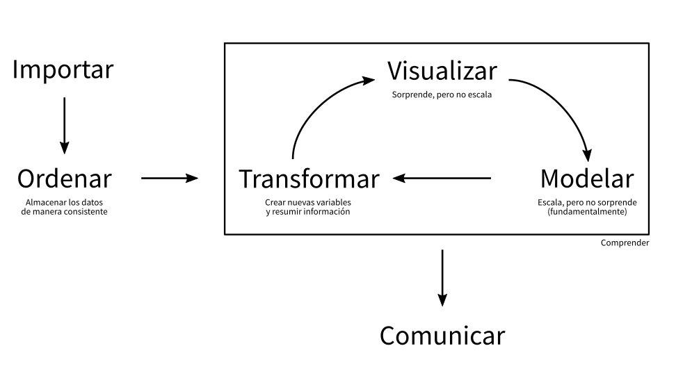
Seguimos con el mismo flujo de datos:

Repaso clase anterior

No puedo explicar sin entender

El Análisis Exploratorio y la Estadística Descriptiva son parte clave para el entendimiento

Escuchar lo que los datos nos hablan

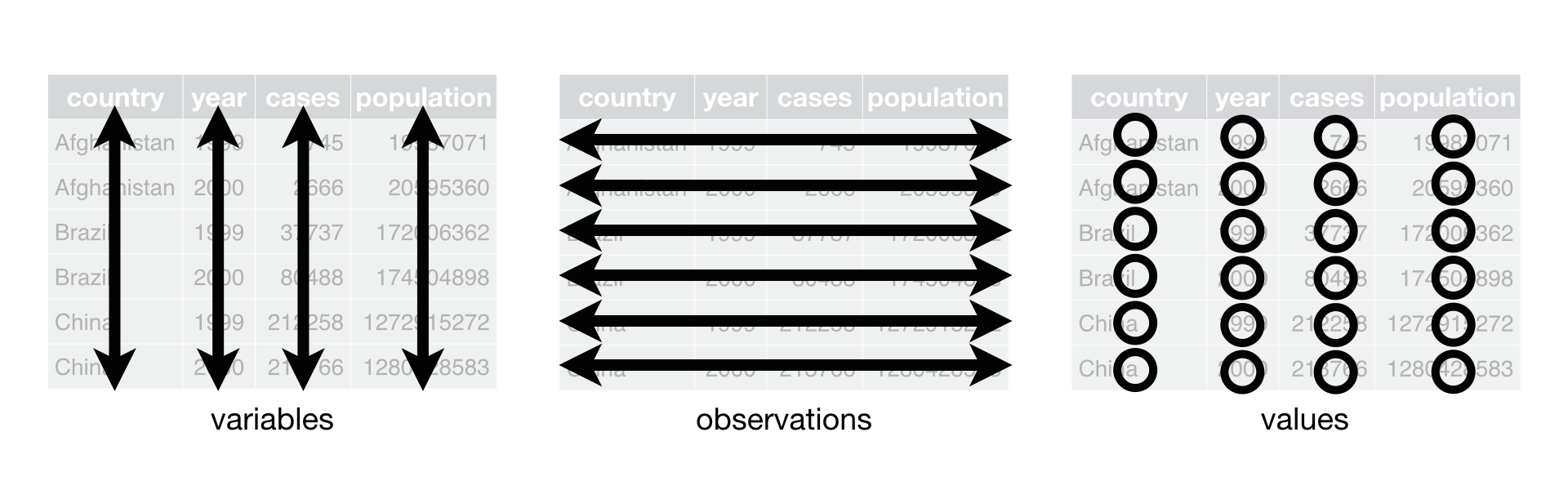
Conceptos

• Una variable es una cantidad, que puede ser medida: estatura, magnitud de un sismo, velocidad de un huracán, etc
• Un valor es un estado de la variable cuando se mide: 1.20 metros, 8° Richter
• Una observación o caso es un conjunto de mediciones -no de la misma variable necesariamente- pero si en un mismo instante y a un mismo objeto.

Conceptos

• Datos tabulados es un conjunto de valores cada uno asociado a una variable y una observación

Conceptos

Análisis Exploratorio de Datos

• Generar preguntas acerca de los datos
• Buscar respuestas visualizando, transformando los datos
• Hacer nuevas preguntas a partir de lo aprendido

Generar conocimiento

Lluvias en la RM

• Cada observación es un registro diario
• Todas las mediciones están registradas en milimetros

Ejercicio 1

• Carga el Tidyverse
• Carga los datos
• ¿Cumple esto con Tidy Data?
• De no cumplir el criterio ordena los datos

Solución Ejercicio 1

library(tidyverse)
library(readxl)

precipitaciones_bruto <- read_excel("data/lluvias.xlsx")
precipitaciones_bruto

## # A tibble: 365 x 44
##    fecha               pp1971 pp1972 pp1973 pp1974 pp1975 pp1976 pp1977
##    <dttm>               <dbl>  <dbl>  <dbl>  <dbl>  <dbl>  <dbl>  <dbl>
##  1 2017-01-01 00:00:00  0          0      0      0      0      0      0
##  2 2017-01-02 00:00:00  0          0      0      0      0      0      0
##  3 2017-01-03 00:00:00  0          0      0      0      0      0      0
##  4 2017-01-04 00:00:00  0          0      0      0      0      0      0
##  5 2017-01-05 00:00:00  0.100      0      0      0      0      0      0
##  6 2017-01-06 00:00:00  0          0      0      0      0      0      0
##  7 2017-01-07 00:00:00  0          0      0      0      0      0      0
##  8 2017-01-08 00:00:00  0          0      0      0      0      0      0
##  9 2017-01-09 00:00:00  0          0      0      0      0      0      0
## 10 2017-01-10 00:00:00  1.60       0      0      0      0      0      0
## # ... with 355 more rows, and 36 more variables: pp1978 <dbl>,
## #   pp1979 <dbl>, pp1980 <dbl>, pp1981 <dbl>, pp1982 <dbl>, pp1983 <dbl>,
## #   pp1984 <dbl>, pp1985 <dbl>, pp1986 <dbl>, pp1987 <dbl>, pp1988 <dbl>,
## #   pp1989 <dbl>, pp1990 <dbl>, pp1991 <dbl>, pp1992 <dbl>, pp1993 <dbl>,
## #   pp1994 <dbl>, pp1995 <dbl>, pp1996 <dbl>, pp1997 <dbl>, pp1998 <dbl>,
## #   pp1999 <dbl>, pp2000 <dbl>, pp2001 <dbl>, pp2002 <dbl>, pp2003 <dbl>,
## #   pp2004 <dbl>, pp2005 <dbl>, pp2006 <dbl>, pp2007 <dbl>, pp2008 <dbl>,
## #   pp2009 <dbl>, pp2010 <dbl>, pp2011 <dbl>, pp2012 <dbl>, pp2013 <dbl>

Solución Ejercicio 1

No cumple con Tidy Data, por lo tanto hay que ordenar

precipitaciones_ordenado <- precipitaciones_bruto %>% 
  gather(anio, precipitacion, -fecha) 

precipitaciones_ordenado

## # A tibble: 15,695 x 3
##    fecha               anio   precipitacion
##    <dttm>              <chr>          <dbl>
##  1 2017-01-01 00:00:00 pp1971         0    
##  2 2017-01-02 00:00:00 pp1971         0    
##  3 2017-01-03 00:00:00 pp1971         0    
##  4 2017-01-04 00:00:00 pp1971         0    
##  5 2017-01-05 00:00:00 pp1971         0.100
##  6 2017-01-06 00:00:00 pp1971         0    
##  7 2017-01-07 00:00:00 pp1971         0    
##  8 2017-01-08 00:00:00 pp1971         0    
##  9 2017-01-09 00:00:00 pp1971         0    
## 10 2017-01-10 00:00:00 pp1971         1.60 
## # ... with 15,685 more rows

Solución Ejercicio 1

¿Puede mejorar? Sí, se puede simplificar

library(lubridate)

precipitaciones_ordenado <- precipitaciones_ordenado %>% 
  mutate(dia = day(fecha),
         mes = month(fecha),
         anio = str_sub(anio, 3, 6)) %>% 
  mutate(dia = ifelse(nchar(dia) == 1, paste0("0", dia), dia),
         mes = ifelse(nchar(mes) == 1, paste0("0", mes), mes),
         anio = as.integer(anio)) %>% 
  unite(fecha, anio, mes, dia, sep = "-", remove = F) %>% 
  mutate(fecha = ymd(fecha)) %>% 
  select(fecha, anio, precipitacion)

Solución Ejercicio 1

Resultado final

precipitaciones_ordenado

## # A tibble: 15,695 x 3
##    fecha       anio precipitacion
##    <date>     <int>         <dbl>
##  1 1971-01-01  1971         0    
##  2 1971-01-02  1971         0    
##  3 1971-01-03  1971         0    
##  4 1971-01-04  1971         0    
##  5 1971-01-05  1971         0.100
##  6 1971-01-06  1971         0    
##  7 1971-01-07  1971         0    
##  8 1971-01-08  1971         0    
##  9 1971-01-09  1971         0    
## 10 1971-01-10  1971         1.60 
## # ... with 15,685 more rows

Ejercicio 2

Filtra los datos a partir del año 2000

Solución Ejercicio 2

precipitaciones_ordenado %>% 
  filter(anio >= 2000)

## # A tibble: 5,110 x 3
##    fecha       anio precipitacion
##    <date>     <int>         <dbl>
##  1 2000-01-01  2000             0
##  2 2000-01-02  2000             0
##  3 2000-01-03  2000             0
##  4 2000-01-04  2000             0
##  5 2000-01-05  2000             0
##  6 2000-01-06  2000             0
##  7 2000-01-07  2000             0
##  8 2000-01-08  2000             0
##  9 2000-01-09  2000             0
## 10 2000-01-10  2000             0
## # ... with 5,100 more rows

Ejercicio 3

Filtra las precipitaciones mayores o iguales a 50mm

Solución Ejercicio 3

precipitaciones_ordenado %>% 
  filter(precipitacion >= 50)

## # A tibble: 29 x 3
##    fecha       anio precipitacion
##    <date>     <int>         <dbl>
##  1 1971-06-20  1971          68.7
##  2 1972-08-12  1972          58.0
##  3 1974-06-29  1974          57.3
##  4 1978-11-16  1978          51.7
##  5 1979-07-26  1979          62.5
##  6 1981-05-30  1981          85.6
##  7 1982-05-12  1982          51.9
##  8 1982-06-26  1982          61.2
##  9 1984-07-04  1984          77.6
## 10 1984-07-10  1984          50.2
## # ... with 19 more rows

Ejercicio 4

Crea una nueva tabla con las precipitaciones mayores a cero

Solución Ejercicio 4

precipitaciones_ordenado_2 <- precipitaciones_ordenado %>% 
  filter(precipitacion > 0)

precipitaciones_ordenado_2

## # A tibble: 2,261 x 3
##    fecha       anio precipitacion
##    <date>     <int>         <dbl>
##  1 1971-01-05  1971         0.100
##  2 1971-01-10  1971         1.60 
##  3 1971-01-11  1971         0.100
##  4 1971-01-22  1971        11.0  
##  5 1971-02-28  1971         0.100
##  6 1971-03-02  1971         0.100
##  7 1971-04-19  1971         0.100
##  8 1971-04-20  1971         4.40 
##  9 1971-04-25  1971         0.100
## 10 1971-05-14  1971         3.60 
## # ... with 2,251 more rows

Ejercicio 5

Grafica la serie de precipitaciones a partir del ejercicio anterior

Solución Ejercicio 5

g1 <- precipitaciones_ordenado_2 %>% 
  ggplot(aes(x = fecha, y = precipitacion, color = precipitacion)) +
    geom_line()

g1

Ejercicio 6

Agrega una línea horizontal para mostrar claramente los registros que superan los 50 mm diarios

Solución Ejercicio 6

g1 <- g1 +
  geom_hline(yintercept = 50, color = "red", linetype = "dashed")

g1

Ejercicio 7

• Agrega el texto “50mm” a la línea de corte (al lado derecho)
• Remueve la leyenda
• Usa el tema white

Solución Ejercicio 7

fmax <- max(precipitaciones_ordenado_2$fecha)

g1 <- g1 + 
  annotate("text", fmax, 50, vjust = -1, label = "50 mm") +
  theme(legend.position = "none") + theme_bw()

g1

Ejercicio 8

• Agrega etiquetas a los ejes del gráfico
• Usa las fechas mínima y máxima como límites del eje x
• Agrega algunas fechas como referencia (i.e intervalos de 5 años o 1825 días)
• Agrega título

Solución Ejercicio 8

fmin <- min(precipitaciones_ordenado_2$fecha)

g1 <- g1 + 
  labs(y = "milimetros de lluvia", x = "año") +
  theme(legend.position = "none", 
        axis.text.x = element_text(angle = 90, hjust = 1)) +
  scale_x_date(date_labels =  "%d-%m-%Y", 
               limits = c(fmin, fmax), 
               breaks = c(fmin, fmin + seq(1825,1825*8,1000), fmax)) +
  ggtitle("Precipitaciones registradas en la RM desde 1971")

Solución Ejercicio 8

g1

Ejercicio 9

• Usa facets_wrap para crear mini gráficos para los años 2009 - 2012
• Recuerda incluir etiquetas en los ejes y título

Solución Ejercicio 9

precipitaciones_ordenado_2 %>% 
  filter(anio >= 2009 & anio <= 2012) %>% 
  ggplot(aes(x = fecha, y = precipitacion, color = anio)) +
  geom_col() +
  facet_wrap("anio", scales = "free_x", ncol = 4) +
  theme_bw() +
  theme(legend.position = "none",
        axis.text.x = element_text(angle = 90, hjust = 1)) +
  labs(y = "milimetros de lluvia", x = "año") +
  ggtitle("Precipitaciones registradas en la RM 2009-2012")

Solución Ejercicio 9

Ejercicio 10

• Obten la suma de precipitaciones por mes en un año a tu elección
• Grafica los resultados

Solución Ejercicio 10

precipitaciones_ordenado %>% 
  filter(anio == 2012) %>% 
  mutate(mes = month(fecha, label = TRUE)) %>% 
  group_by(mes) %>% 
  summarise(pmes = sum(precipitacion)) %>% 
  ggplot(aes(x = mes, y = pmes)) +
  geom_col() +
  theme_bw() +
  theme(legend.position = "none",
        axis.text.x = element_text(angle = 90, hjust = 1)) +
  labs(y = "milimetros de lluvia", x = "año") +
  ggtitle("Precipitaciones registradas en la RM en 2012")

Solución Ejercicio 10